Deep dive: Auto scaling response times on Amazon ECS
When traffic to your application spikes, how quickly auto scaling responds determines whether users see fast responses or timeouts. Amazon Elastic Container Service (Amazon ECS) service auto scaling handles this by adjusting the number of tasks in a service to meet demand. It includes predictive scaling for recurring patterns, scheduled scaling for known events, and target tracking. With target tracking, you set a target value for a metric such as average CPU or memory utilization.
Many teams rely on target tracking to keep their services responsive as demand rises and falls. By default, ECS publishes CPU and memory utilization every 60 seconds, a resolution well suited to steady, gradual traffic. For applications that experience sudden spikes, the default 60-second resolution might not be responsive enough, and a service can take several minutes to detect the change and add capacity. This leads some teams to over-provision to stay ahead of demand.
Amazon ECS now detects and responds to load changes faster with high-resolution (20-second) CPU and memory utilization metrics for target tracking, in addition to the default 60-second resolution. With higher-resolution metrics, capacity arrives much closer to when demand rises. Your service spends less time serving slow or failing requests during a spike, and you have less need to over-provision for headroom you rarely use. ECS also optimized the metric publishing path for high-resolution metrics, so each measurement reaches the scaling policy sooner.
In the AWS benchmarking published with the launch announcement, time to trigger scale-out fell 76 percent, from 363 seconds to 86 seconds. The time from triggering a scale-out to placing the new tasks fell 72 percent, from 386 seconds to 109 seconds. The first number is how long the service takes to decide to add capacity. The second is how long until the new tasks are running. Reacting faster on both counts can mean lower latency during a spike, fewer failed requests, and less capacity sitting idle as a safety margin.
Why scaling speed matters
Target tracking is the most straightforward scaling policy to set up. You choose a target for a metric, such as 60 percent average CPU utilization, and ECS adds or removes tasks to keep the service near it. Because it’s fully managed, you don’t configure alarms or maintain step-scaling rules, and it works well for most workloads. However, for workloads where load rises suddenly, publishing the utilization metric every 60 seconds can delay scale-out. In such cases, teams provision extra capacity to handle the load during the scale-out period. The extra capacity goes unused whenever load is below peak.
This is why scaling speed matters. The faster a service responds to rising load, the less capacity it needs to hold in reserve, and the more consistent the experience it delivers to customers during a spike.
What changed
Two changes work together to shorten the response time.
Higher-resolution metrics – ECS can now publish CPU and memory utilization every 20 seconds, in addition to the default 60-second resolution. AWS Application Auto Scaling target tracking consumes these high-resolution metrics, so the confirmation window now spans seconds, and ECS can decide to scale out much sooner.
A lower-latency publishing path – More frequent data points help only if they also arrive quickly. For the high-resolution metrics, ECS optimized the path that carries a measurement from a running task to an available Amazon CloudWatch metric. It publishes each value with far less delay, so the policy sees recent load almost as soon as it happens.
Together, these two changes give the policy more frequent and more recent data, so it detects a load change and adds capacity far sooner.
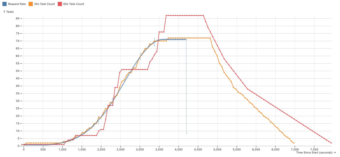
The following figure shows the effect as request rate rises and falls, comparing a service scaling on 20-second metrics with one scaling on 60-second metrics. The service on 20-second metrics follows the request rate closely. The service on 60-second metrics lags behind, rising in large steps, overshooting the peak, and releasing capacity slowly after demand falls. With faster metrics, capacity stays matched to the load as it rises, and the service keeps up.
Figure 1: Running task count compared to request rate on AWS Fargate, 20-second and 60-second metrics
Benchmarking faster auto scaling
This section describes how we tested faster auto scaling against realistic workloads on both AWS Fargate and ECS Managed Instances, and what the results show.
How we measured it
The scaling numbers in the introduction measure the scaling mechanism itself, timing how quickly a policy triggers a scale-out and how long until the new tasks are running. The benchmarks in this section measure something different, which is how a real application behaves under changing load. To do this, the AWS Benchmarking team performed a standardized, automated load test that compared the same workload and configuration with standard 60-second metrics and with 20-second high-resolution metrics.
This benchmarking test used the following setup.
- Compute: Amazon ECS on AWS Fargate and on ECS Managed Instances, using amd64 (x86-64) tasks of 1 vCPU each, in the US West (Oregon) AWS Region (us-west-2).
- Scaling policy: Target tracking on average CPU utilization at a 60 percent target, scaling between 1 and 128 tasks.
- Load generation: k6 driving demand as a ramping arrival rate that follows a normal (bell) curve, updated every 30 seconds, with up to 32,000 virtual users and a 90-second request timeout.
- Statistics: Each metric is reported as a median across 24 runs per workload profile.
We use three workload profiles that stand in for different kinds of real applications and failure modes. In each, every request performs the same work. That work is a Monte Carlo estimate of the variance and median of 100,000 samples from a truncated normal distribution, implemented idiomatically in each language. The profiles differ in how the application starts up, how expensive each request is, and how demand changes over time:
- Rust, gradual ramp – A fast-starting service under steady, predictable growth. Think of an API whose traffic climbs through the business day. It uses the Rocket web framework, which boots quickly, and does about 1 ms of work per request. Demand ramps up over 30 minutes and back down over 30 minutes, from roughly 200–20,000 requests per second. This is our primary profile for steady-state responsiveness. The failure mode is falling steadily behind a smoothly rising load.
- Java, repeated spikes – A slow-starting service hit by repeated bursts. New tasks need JVM warm-up before they can serve traffic, so this is the worst case for cold starts. While new capacity warms up, users can see errors and timeouts. It does about 10 ms of work per request across three 10-minute-up, 10-minute-down cycles (roughly 40–4,000 requests per second).
Node.js, steady growth – A typical web service that grows over a long window, then stops. Demand stays low for 10 minutes, ramps up over 50 minutes, holds for 10 minutes, then drops abruptly from roughly 20–2,000 requests per second. Each request does about 15 ms of work. This represents production traffic that builds over time, and it tests how promptly a service releases capacity after demand disappears.
The primary metric, service-level agreement (SLA) breach time, is the total duration of 6-second windows in which more than 10 percent of requests failed. A request counts as a failure if it takes longer than 2 seconds, returns an error, or is dropped. The 2-second bar is a deliberately strict SLA threshold. Requests aren’t actually timed out until 90 seconds. This reflects how long real users would have experienced problems, not only how quickly the service scaled. We also report scale down duration, the time to return to baseline capacity after the load drops.
Time spent breaching SLA
The following table shows SLA breach time (median, in seconds) with standard 60-second metrics and with 20-second high-resolution metrics.
SLA breach time (seconds)
| Workload profile | Fargate: 60s → 20s | Managed Instances: 60s → 20s |
| Rust, gradual ramp | 2,013 → 633 (69% lower) | 1,692 → 30 (98% lower) |
| Java, repeated spikes | 2,232 → 1,131 (49% lower) | 1,593 → 750 (53% lower) |
Node.js, steady growth | 750 → 3 (99% lower) | 969 → 102 (89% lower) |
On the gradual-ramp profile, SLA breach time on Fargate fell 69 percent, from 2,013 to 633 seconds (about 34 minutes down to 11), and Managed Instances fell 98 percent, from 1,692 to 30 seconds. These are medians across 24 runs, measured as described in “How we measured it”.
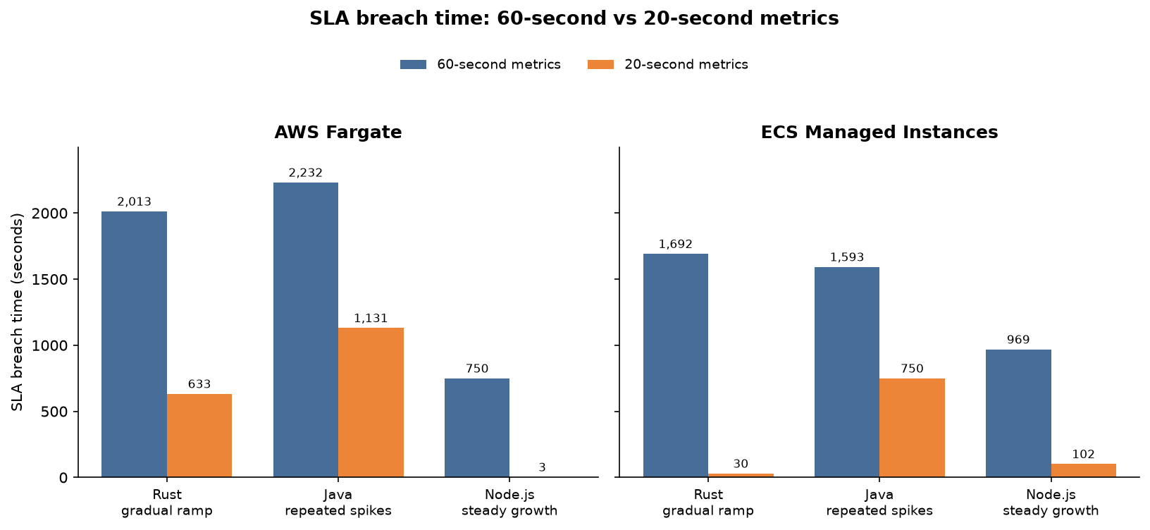
Figure 2: SLA breach time by workload profile, 60-second and 20-second metrics
Faster scaling also made the results more consistent. With 20-second metrics, running the same test repeatedly gave nearly the same result each time, while 60-second metrics varied much more.
Why Managed Instances scale even faster
On ECS Managed Instances, ECS runs several tasks per instance, so it can place a new task on an instance that’s already running and has spare capacity. In that case, there is no new instance to provision, and the container image is often already cached on that instance from earlier task launches. This is why Managed Instances show the largest SLA breach-time improvements, particularly on the gradual-ramp profile. On Fargate, each task runs in its own dedicated, isolated environment that ECS provisions on demand. ECS pulls the image into that environment before the task can start, which adds time to each scale-out step.
The faster metrics speed up the scaling decision equally for both compute options. Managed Instances act on that decision sooner, which is why their 20-second gains are the largest.
Returning capacity after the surge
The same higher-resolution, lower-latency metrics also help on the way down. Tasks that keep running after demand has dropped add cost without serving load, so a shorter scale-down duration can reduce spend. The following table shows scale down duration (median, in seconds).
Scale down duration (seconds)
| Workload profile | Fargate: 60s → 20s | Managed Instances: 60s → 20s |
| Rust, gradual ramp | 1,943 → 42 (98% lower) | 2,343 → 37 (98% lower) |
| Java, repeated spikes | 4,120 → 2,102 (49% lower) | 2,091 → 1,679 (20% lower) |
Node.js, steady growth | 3,853 → 2,803 (27% lower) | 3,680 → 1,878 (49% lower) |
For the gradual-ramp profile, scale down fell from 1,943 seconds (Fargate) and 2,343 seconds (Managed Instances) to 42 and 37 seconds. That’s a drop from over half an hour to under a minute. These are medians across 24 runs, measured as described in “How we measured it”. The bursty Java and steady-growth Node.js profiles improved less (a 20–49 percent reduction), because these workloads stop traffic more abruptly, leaving a shorter window for faster metrics to make a difference.
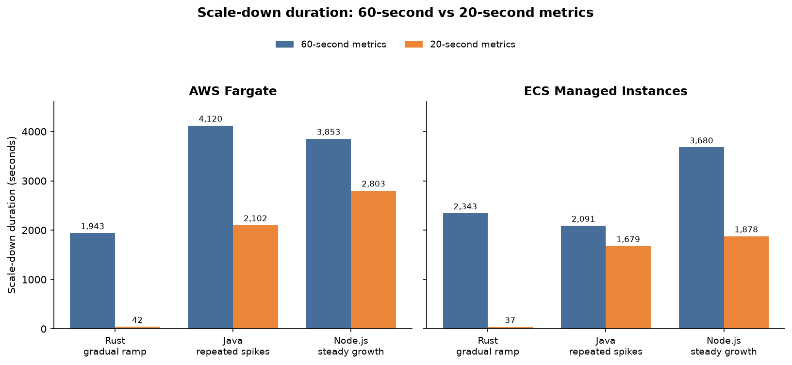
Figure 3: Scale down duration by workload profile, 60-second and 20-second metrics
How faster scaling affects your application
The most important result is the drop in SLA breach time. SLA breach time is the time during which end users experienced slow or failed requests, and faster scaling brought it down significantly, because:
- The service doesn’t fall as far behind. Acting sooner keeps it from being overwhelmed in the first place, and preventing that’s worth more than recovering from it later.
- The time saved adds up at each step. A large jump in traffic is handled over several scaling steps, and faster reaction saves time at every step, not only the first.
- Each decision uses more recent information. More recent measurements let the service size itself more accurately, so it adds fewer extra tasks and makes fewer corrections.
Faster auto scaling also improves scale down. A service that tracks demand closely builds up fewer extra tasks to remove, and more frequent measurements let it lower capacity sooner with less risk of cutting too far.
When to use this
High-resolution auto scaling helps most when scaling speed affects customer experience or cost:
- Bursty or spiky workloads, such as APIs behind sudden traffic or event-driven services.
- Latency-sensitive applications, where even a short period of degradation is a poor experience.
- Services you over-provision today to survive scaling lag. With faster scaling, you can reduce that baseline and lower cost.
20-second metrics are billed as CloudWatch high-resolution metrics. They are best turned on where they deliver a clear benefit, rather than on every service by default. Use them where scaling lag is affecting latency or availability, or where you over-provision to compensate for it. For stable, slowly changing workloads, the default 60-second metrics are usually sufficient.
How to turn it on
To turn on faster auto scaling, complete two steps in the ECS console or with the AWS Command Line Interface (AWS CLI), AWS CloudFormation, or the AWS SDKs:
- Turn on 20-second metrics for CPU and memory on your service (on the console, under Monitoring configuration when you create or update the service). For an existing service, do this first and let the deployment finish so the service begins emitting high-resolution metrics.
- Attach a target tracking policy that uses one of the two new predefined high-resolution metrics:
ECSServiceAverageCPUUtilizationHighResolution– Average CPU utilization at 20-second resolution.ECSServiceAverageMemoryUtilizationHighResolution– Average memory utilization at 20-second resolution.
You can use high-resolution auto scaling across all ECS compute options, including AWS Fargate, ECS Managed Instances, and Amazon Elastic Compute Cloud (Amazon EC2). Container Insights isn’t required. For a step-by-step walkthrough with console and CLI examples, see the launch blog post and the faster auto scaling documentation.
There’s no additional charge for the feature or for the default 60-second CPU and memory metrics. Publishing them at 20-second resolution makes them high-resolution metrics, which CloudWatch bills per metric. See the Amazon CloudWatch pricing page, and weigh the metric cost against the buffer capacity you no longer need to keep on hand for slow scaling.
Other scaling options
High-resolution CPU and memory metrics make reactive target tracking much faster, but they are one tool among several, and the strongest setups combine them:
- Predictive and reactive scaling together. Predictive scaling learns recurring daily or weekly patterns and adds capacity ahead of a known ramp. A busy period therefore starts already scaled. Reactive target tracking then handles whatever the forecast didn’t. An unexpected spike on top of the expected curve is a typical example. Using both means you can handle sudden changes in load, and predictable traffic is handled before it arrives. Scheduled scaling covers known one-off events such as a product launch or sale.
- Custom metrics, at your own resolution. Not every service scales best on CPU or memory. Your load might be better reflected by another signal, such as Amazon Simple Queue Service (Amazon SQS) queue depth, requests per target, or a business metric. You can publish that signal to CloudWatch as a custom metric at the resolution you choose, including high resolution, and use it with target tracking today. So faster scaling isn’t limited to CPU- or memory-bound services, and you can get a fast reactive signal from the metric that drives your workload.
Conclusion
High-resolution 20-second metrics and a lower-latency publishing path shorten the time Amazon ECS takes to react to a load change. In our benchmarks, this reduced SLA breach time and shortened the scale-down duration to under a minute on the gradual-ramp profile across both Fargate and Managed Instances. The largest gains were on Managed Instances, where new tasks start on warm, shared capacity. Because a service that reacts sooner doesn’t fall as far behind, the time it spends breaching its SLA can improve by far more than the reaction time alone. Paired with predictive scaling and custom metrics, target tracking gives you a fast, fully managed response to both expected and unexpected changes in load.
To get started, see the faster auto scaling documentation and the Amazon ECS service auto scaling documentation. For what is coming next, see the AWS Containers roadmap on GitHub. We welcome your feedback through AWS re:Post for ECS or your usual AWS Support contacts.
About the authors
原文:https://www.a8q9.cn/en/article/deep-dive-auto-scaling-response-times-on-amazon-ecs-c8feae.html